
Neural Nets & Tensor Flow
I had gotten curious to Tensor Flow from Adrian Colyer’s morning paper. Having a bit of time, I therefore decided to renew my almost 30 year old acquaintance with neural networks. At the end of the eighties I bought all the books but memories were dim; at the time it was no feasible for any serious problems.
Today, with computers a million times faster the story is different. Especially with TensorFlow. TensorFlow is a large mathematical library that can execute the tensor formula’s remotely and on special hardware like Graphic Processing Units (GPU) and special Tensor Processing Units (TPU), reaching speeds a super computer of only a few years ago would have been jealous. (Tensors, by the way, are n-dimensional matrices. I.e. scalars, vectors, matrices, volumes, and so on.)
I started with the TensorFlow introductory tutorial and that meant Python. Somehow Python and I will never really become friends. I therefore tried the Java API but that was a result of either a Python programmer illegally practising Java or a junior trainee that missed the day that Java was taught at university. Stupid that I am, I set out to create my own wrapper.
Now, for the kids among us, don’t try this at home. Never write a library (wrapper) when you’re not intricately familiar with the subject at hand. Vaguely aware of this idea I decided to first do some refreshing. Ok, maybe get some fundamentals since I never deep dived in the math of neural networks 30 years ago. (Looking back in my old books, surprisingly little has changed though.) I found an online book about neural networks that looked pretty thorough. Better, it was referred to from the TensorFlow site. Dumb as I am, I decided to write my own Java classes and not follow the Python code, telling myself it was a good learning exercise. And boy, was I right. This blog recounts my adventures. Follow along at your own peril. For extra points, use the Java 9 JShell to make your own neural network with multiple layers and teach it a NAND gate.
Quick Guide into Neural Nets
A neural net is number of layers of neurons. Output of one neuron is relayed to the input of other neurons in the next layer. The other neurons weigh and bias their inputs and then decide on an output value using a transformation function. This output value is either the final result, in the case of the output layer, or it is fed into the next layer.
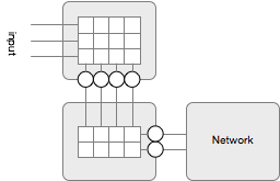
I could now show a classic traditional picture of a neuronal network but that just does not work well for me. All those crossing lines are hurting my esthetic feelings. My mental model of a neuronal network is therefore the following picture:
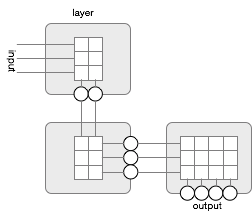
With a simple neuronal network like this you could make weights and biases that would, for example, show the number of one bits in the input on the output.
 Input   Output
 000     0000
 001     0001
 010     0001
 011     0010
 100     0001
 101     0010
 110     0010
 111     1000
The picture shows a 3 layer network. (In the book this would be 4 since they count the input as a layer.) It is a 3-2-4 network. Each layer has an input cardinality and an output cardinality. We call the input cardinality #in and the output cardinality #out, you will see them used quite often so try to understand how they relate.
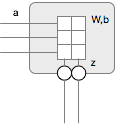
The picture has a table where each cell holds the weight of an input j to a neuron k in that layer. Not shown in the picture is the bias that each neuron also has. For the input, a neuron multiplies each input with its special dedicated weight and then sums them together after which it adds the bias. The result is called z, which we can call the raw input value.
I never really had any experience with matrix multiplications so I had to follow some courses on Khan academy to get up to speed. Amazing stuff! When you structure your matrices and vectors correctly, you can do most of this weight multiplication and bias addition in two operations. If W is the weight matrix, b the bias vector, and a is the input vector then we can say:
z = Wa + b
Wow, deceptively simple. #not. Matrix multiplication is clearly not my grandmother’s multiplication so I did some struggling. For other souls that never wrestled with it a short primer on matrix multiplication. Feel free to skip if you did pay attention during class.
Short Primer on Matrices
When you multiply 2 matrices A * B you end up with a matrix C. C gets its number of rows from A’s rows and the number of columns from B’s columns. Oh yeah, the number of columns of A must equal the number of rows of B to make a multiplication possible.
  C.rows == A.rows
  C.cols == B.cols
  A.cols == B.rows
Clearly then, A * B != B * A. It is very important to watch the cardinality of the matrices and the order as I learned in this exercise.

A matrix A(#a,m) and B(#b,j) results in C(i,j) for i in 0..#a, and j in 0..#b. Each entry is given by multiplying the entries A(i,k) (across row i of A) by the entries B(k,j) (down column j of B), for k in 0..m, and summing the results over k. If this looks complicated, suggest you use the Khan academy and checkout multiplication. Just remember, basically the incoming values are multiplied with all the cells and summed to create an output value.
Weight Matrix
In this case, a is a vector with the input values. A vector is actually also a matrix with shape (#in x 1). (They are both tensors.) That is #in rows, and 1 column. So how should we store the weights in W?
If W is shaped (#in x #out) then one cannot easily multiply it with a which is shaped (#in x 1). That is, (#in x #out) * (#in x 1) is malformed since the columns of W (#out) do not match the rows of a (#in). Therefore, we should make W a matrix shaped (#out x #in). Now Wa is a well formed multiplication.
W( #out x #in ) * a( #in x 1) => z(#out x 1)
The dimensions of z are exactly the dimensions we need as input to our neurons! Magic!
A concrete example where we have a 3-2 layer. I.e. we get 3 inputs and create 2 outputs:
                                a(3x1)
                                0.50
                                0.10
                                0.30
          W(2x3)
          0.50   -0.5   0.30    0.29  z(2x1)
          0.10    0.2  -0.10    0.04
JShell
You can try this out in the Java 9 JShell! I am using the org.jblas as matrix library you can find on Maven Central.
  jshell> import org.jblas.*
  jshell> FloatMatrix W = FloatMatrix.valueOf("0.5 -0.5 0.3; 0.1 0.2 -0.1")
  W ==> [0.500000, -0.500000, 0.300000; 0.100000, 0.200000, -0.100000]
  jshell> FloatMatrix a = FloatMatrix.valueOf("0.5;0.1;0.3")
  a ==> [0.500000; 0.100000; 0.300000]
  jshell> W.mmul(a)
  $6 ==> [0.290000; 0.040000]
If you use the JSHell, it is easiest to call up an editor with /edit. You can then paste the code and Accept it. My MacOS shell was not very good in accepting pasted code. Later you can do /edit Network or /edit MiddleLayer to edit the class.
Output
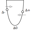
Every neuron has a function that takes the weighted and biased raw input z and turns it into an output. The first neuronal models used a threshold function. If the weighted input of a row in z was above a threshold, the corresponding output was 1 and otherwise 0. The diagram for this neuron transform function is:
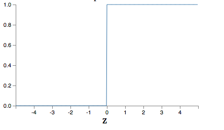
Unfortunately, such a function has the problem that a network can easily get unstable. A small change in weight, bias, or input can have a tremendous effect on the output, especially with multiple layers or when the raw input z is close to the threshold. Therefore, the sigmoid function, to impress we’ll use the fancy symbol σ for the name of this function, works much better because it has a gradual threshold. It has the following graph:
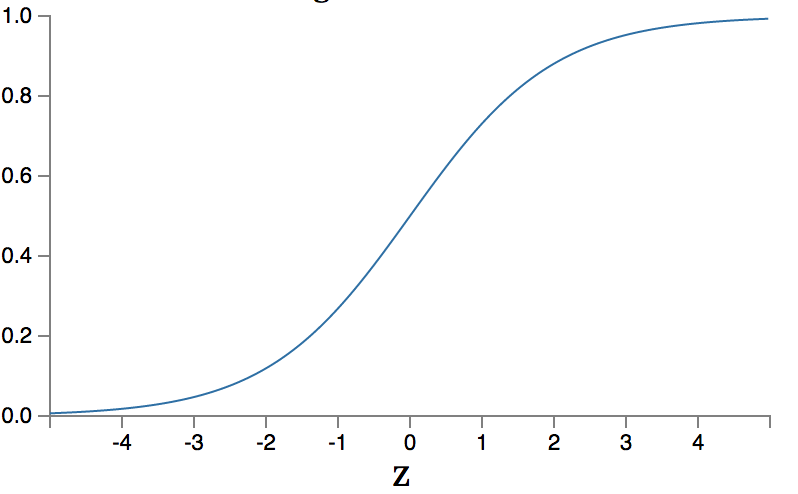
Or in formula form:
It should be clear, but to be sure. z is a vector so the function σ(z) must accept a vector and return one.
API
As always, first the API! Never without an API is the primary lesson I learned as a developer. Always API, even if what we’re doing seems trivial.
The API for a layer looks like:
interface Layer {
	FloatMatrix activate(FloatMatrix x);
}
Middle Layer
The Middle Layer needs to transform the input vector a to an output a’, which is the input for the next layer. For this transformation we need the following class:
class MiddleLayer implements Layer {

	Layer		next;
	FloatMatrix	W; // (#out x #in)
	FloatMatrix	b; // (#out x 1)

	MiddleLayer(int in, int out, Layer next) {
		this.W = FloatMatrix.rand(out, in);
		this.b = FloatMatrix.rand(out, 1);
		this.next = next;
	}

	@Override
	public FloatMatrix activate(FloatMatrix aIn) {
		FloatMatrix z = W.mmul(aIn).addi(b); // #out x 1
		return next.activate(σ(z));
	}

	static final FloatMatrix ONE = FloatMatrix.scalar(1);
	FloatMatrix σ(FloatMatrix vector) {
		return ONE.div(ONE.add(MatrixFunctions.exp(vector.neg())));
	}
}
We initialize the W matrix and the b vector with random numbers between 0..1. This works better when we later train the network.
The activate method propagates the result of that layer, the output value a’, to the next layer, and the last ‘layer’ is actually the network that will just return. This value at the end is actually the prediction made by the layers.
Programming the Layer
We use a Network class to hold the different layers together:
  	public class Network implements Layer {
	Layer input;

	public Network(int... shape) {
		assert shape.length > 1;
		int last = shape.length - 1;
		this.input = this;
		for (int x = last; x > 0; x--) {
			this.input = new MiddleLayer(shape[x - 1], shape[x], this.input);
		}
	}

	@Override
	public FloatMatrix activate(FloatMatrix x) {
		return x;
	}
  	}
Notice that the Network objects act as the last layer so we can take special action and let the Middle Layer be just concerned about being, eh, a middle layer. This is generally a sign of a good cohesive design if you do not need a special case.
The Network constructor creates a number of linked layers. The #out of the previous layer’s output is the #in of the next layer. For a network of 3-4-2, i.e. new Network( 3,4,2), The layers would look like:
Layer input = new MiddleLayer(3,4,new MiddleLayer(4,2, this)); // don't paste this in JSHell
Or as a picture:
Testing
Clearly this network will return a value but it will be random because we’ve initialized the weight and the bias to random numbers. No training has taken place. However, from an infrastructure point of view it is nice to get a short test case.
In the shell we can now create a simple network and ask for the activation.
> Network n = new Network(2,1)
n ==> Network@63440df3
> n.input.activate( FloatMatrix.valueOf("1;1") )
$33 ==> [0.838629]
> n.input.activate( FloatMatrix.valueOf("1;0") )
$34 ==> [0.715076]
Clearly not very useful values! But that was to be expected since we’ve not trained the network yet. However, we know that at least we got the matrix dimensions right since there is no exception. (That did take some effort!)
Training a Network
To train the network we need provide inputs and the expected outputs. A training algorithm will then adjust the weights W and the biases b. As always, there are many ways to skin a cat. The TensorFlow library has many different algorithms that implement different training algorithms but they are all implemented in Python.
In this example we use a back propagation algorithm since it is pretty straightforward.
Back propagation means that we predict a value just like with the activate method. However, when we are at the last Middle Layer, we calculate an error δ. (Unicode characters are great!), a vector of shape (#out x 1). I.e. we have an error value for each separate neuron in δ.
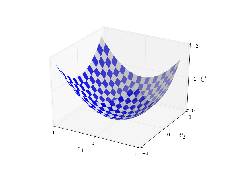
To calculate δ we need a cost function whose value depends on how far off we are from the goal, the expected value. We then try to find a change in W and b that moves us to a place that has a (slightly) lower cost. It is a bit like being on a n-dimensional plane and for each dimension you try to make a tiny little step down until you finally reach the lowest place. Visually for 2 dimensions it is a valley. Consider you’re somewhere on the slopes, then as long as you go a little bit down in the left and right direction you should get to the lowest point in the valley finally.
If x is the input vector from a training set and y(x) is the desired value then a cost function that works well for our network is (a’ is the calculated output value, the input value for the next layer):
C(a') = ( y(x) - a' )^2
Clearly, we’ve reached 0 cost when y(x) = a. The trick now is to change W and b in such a way the error decreases in a controlled way. The algorithm that is used here is called gradient descent. For each neuron, it calculates where it is on the cost curve and then tries to establish the direction to move the weights and bias to that makes the cost a bit less so we end up at zero cost.
How does it know that direction? Well, it can derive the cost function and see what the direction of the curve is for the current value C(a’). If the derivative is positive at a’ (curve goes up) then we want a’ to be a bit smaller so we move left and thus down on the cost curve, if the derivative is negative (line curves down), we should move to the right and we therefore want a’ to increase a tad. Remember your calculus?
The derivative of ( y(x) - a' )^2 on a' is 2( y(x) - a') ~ y(x) - a'. We can ignore the constant 2 since we’re looking for the direction to move, not an absolute value. We therefore define the derived cost of a’ when we know the predicted value a’ and the expected value x:
ΔC = a' - y(x)
However! We’re not there. The sigmoid function σ could throw another wrench in our calculations since it could also reverse the direction. I.e. a positive change in W might be turned into a negative change by the neuron function we use. (Not for the sigmoid, but it could for another function.) We therefore must also calculate the derivative of the σ function and multiply this with ΔC to make sure we actually move in the desired direction when we change W and b. Therefore:
ΔC = a' - y(x)
Δa = Δσ(z)
δ = ΔC x Δa   // NOT a matrix multiplication but multiplies per row, like δ[i] = ΔC[i] x Δa[i]
To ensure that we make small steps so that we do not overshoot local minima in our cost valley, or start to oscillate, we have a factor η. This is small value that controls the learning rate. The higher this factor η, the bigger the steps down the cost valley but the easier it will overshoot. I.e. a step could become so big that you step across the bottom of the valley straight to the other side.
The sign of δ now ensures that any change we make to W and b will actually move us in the right direction to lower the cost function. The actual value is not so relevant because we cannot make big steps anyway. Each training step should only marginally modify W and b, it is the repetition and all the other samples that then statistically (well stochastically) moves the W and b to values so that the cost decreases.
We now can calculate the delta to W and b. For W we multiple the error with the input because the weights are multiplied. For b we just add the error since the bias is only an offset.
ΔW = η(δ * a.transpose())  // (#out x 1) * (#in x 1).transpose(1 x #in) = (#out x #in)
Δb = ηδ
W = W + ΔW
b = b + Δb
This described the last Middle Layer. However, the other Middle Layers are very similar. The only difference is how they get their ΔC or cost function. For the last layer it was clear, the training set provides us with a value. The earlier layers do not have a provided value, we therefore need to calculate the ΔC for the previous layer by doing a reverse transformation through W from our error δ. We need some more matrix magic here. To go backwards through a matrix we can transpose it and then multiply it with the value.
ΔC = W.transpose() * δ
Transpose exchanges the columns and the rows. This is necessary to line up the matrix multiplication with the error δ that has a shape of #out x 1. I.e. the shapes are as follows
W(#out x #in).transpose()(#in x #out) * δ(#out x 1) => (#in x 1)
Clearly, the result ΔC is a vector that has the proper output size of the previous layer as one can expect. We ignore the bias in this case since we work with derivatives and the bias is a constant.
To summarize. We’ve defined the layers recursively. Each layer calculates an activation util we reach the last layer, which in our case is the Network object. When we reach the network, we calculate the error ΔC based on the cost function and the expected value. This value is returned as the next layer’s ΔC. The previous layer then calculates its error δ from the next layer’s ΔC. It adjusts the weights, and the returns its ΔC which is the error transformed backwards to its input.
In an action diagram:
Implementation Learning
To structure this properly we implement a learn() method in Layer.
interface Layer {
	FloatMatrix activate(FloatMatrix aIn);
	FloatMatrix learn(FloatMatrix aIn, FloatMatrix y, float η);
}
The learn() method returns the ΔC for the caller. Since the last ‘layer’ is our Network object, we can calculate the final ΔC in the Network class:
@Override
public FloatMatrix learn(FloatMatrix aIn, FloatMatrix y, float η) {
	// ΔC = a - y(x)
	return aIn.sub(y);
}
For the middle layer, the work is a bit more complex but not too bad. After all this is the heart of our training algorithm. So add the following method to the MiddleLayer class that implements the calculations:
@Override
public FloatMatrix learn(FloatMatrix aIn, FloatMatrix y, float η) {

	FloatMatrix z = W.mmul(aIn).add(b);
	FloatMatrix aOut = σ(z);

	FloatMatrix ΔC = next.learn(aOut, y, η);

	// δ = ΔC x Δa
	FloatMatrix Δa = Δσ(z);
	FloatMatrix δ = ΔC.mul(Δa); // not matrix mmul!!
	FloatMatrix ΔW = δ.mmul(aIn.transpose()).mul(η);
	W.subi(ΔW);
	FloatMatrix Δb = δ.mul(η);
	b.subi(Δb);

	return W.transpose().mmul(δ); // for previous layer ΔC
}
The only thing missing is the derivative of the σ(z) function. Surprise! That sigmoid function actually has a handy and very simple derivative.
σ(z) * (1 - σ(z))
You can add the following method to the MiddleLayer class.
FloatMatrix Δσ(FloatMatrix z) {
	return σ(z).mul(ONE.min(σ(z)));
}
Training
All that is left is a training function that takes as input a set of inputs and a set of expected values. For this you can add the following to the Network class:
void train(int iterations, float η, float[][] trainX, float[][] trainY) {
	for (int i = 0; i < iterations; i++) {
		FloatMatrix x = new FloatMatrix(trainX[i % trainX.length]);
		FloatMatrix y = new FloatMatrix(trainY[i % trainX.length]);
		input.learn(x, y, η);
	}
}
Testing 2
Let’s train our network to be a NAND gate. A NAND has 2 inputs and one output.
> Network n = new Network(2,1);
> n.train( 10000, 0.1f, new float[][] { {0,0}, {0,1}, {1,1}, {1,0} }, new float[][] { {1}, {1}, {0}, {1} });
> System.out.println(n.input.activate( FloatMatrix.valueOf( "0;0" )));
[0.999913]  // ~ 1
> System.out.println(n.input.activate( FloatMatrix.valueOf( "0;1" )));
[0.984902]  // ~ 1
> System.out.println(n.input.activate( FloatMatrix.valueOf( "1;1" )));
[0.271314]  // < 0.5
> System.out.println(n.input.activate( FloatMatrix.valueOf( "1;0" )));
[0.984954]  // ~ 1
If we round the output then we actually have taught the network a NAND gate! You can train the network longer to see the outputs go to 1 and 0.
Conclusion
Welcome to the wonderful world if neural networks. The enormous strides that are being made in this area will influence how we write software tomorrow. Don’t be fooled by the simplicity of this network. Yes, it is slow to train because it is written to explain the principles. With TensorFlow, training of even complex networks is nowadays doable at acceptable cost.
It is this enormous speedup that allow today’s networks to perform their impressive feats.
Thanks for Michael Nielsen for both his book and the nice pictures on his website that I shamefully ‘borrowed’.